One evening I went out to the curling club for a few hours and, according to the electronic sign over the highway, three people died on Wisconsin roads while I was there.
There are more than 4 million miles of roads in the United States, and 210 million licensed drivers. That’s a lot of opportunities for things to go wrong. And they do: from 2010 through 2013, there were more than 120,000 fatal vehicle accidents in the US, according to the NHTSA’s Fatality Analysis Reporting System (FARS).
There’s probably an intersection, turn, or merge point near you where you’re used to seeing cars sitting in the shoulder with their hazard lights on. But do some stretches of road actually have more fatal accidents than others? And if there are dangerous locations, where are they?
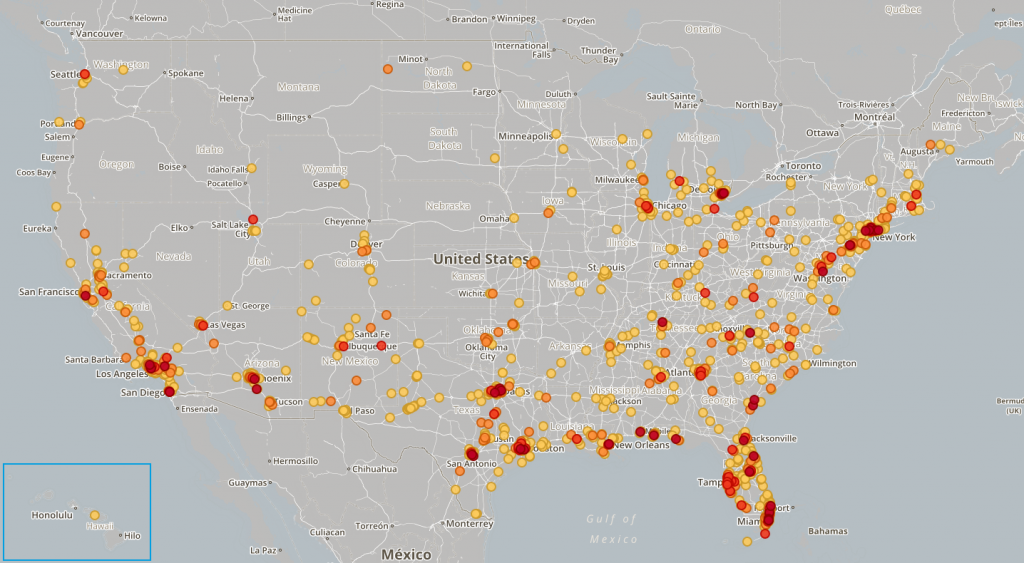
We decided to use MIOedge’s machine learning capabilities and the FARS data to find out. Accident Explorer is an app that finds potentially meaningful clusters of fatal crashes from the 2010-2013 FARS data and displays them on a map using LeafletJS and Mapbox. It’s also a simple demo of our unsupervised machine learning clustering technology.
Before you read on to find out how Accident Explorer finds fatal accident clusters, go ahead and look at all the roads that you and your loved ones regularly drive on. We get it.
Accident Explorer
The foundation of Accident Explorer is the clusters, which identify fatal vehicle accidents that occurred in unusually close proximity. We originally planned to display all fatal accidents on the map and highlight the clusters; when we actually tried it, the browser invariably broke down. Too many points on the map.
So we decided that the map would only show the clusters that we thought were meaningful: clusters of three or more accidents. This made creating a solid algorithm for clustering the data even more important, since users wouldn’t be able to see the unclustered points.
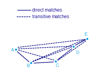
When MIOedge clusters data, it uses transitive matching. With transitive matching, if two pieces of data don’t match when compared directly, they’re matched anyway if they can be connected via direct matches with other pieces of data.
Say we have points A, B, C, D, and E. And using direct matching, we find that A=B, B=C, C=D, and D=E. These are the only direct matches.
But these direct matches, when used with transitive matching, mean that every point matches every other point:
Creating the cluster algorithm
For the first version of Accident Explorer, we started out by considering a popular clustering algorithm named DBSCAN (Density-Based Spatial Clustering of Applications with Noise).
DBSCAN does clustering using two parameters: ε (epsilon), a distance, and K, a minimum neighbor count.
So consider a random fatal vehicle accident, which we’ll call A. DBSCAN considers every accident that took place within ε of A to be A’s neighbor. If A has at least K neighbors, then A and all its neighbors are clustered.
This is the start of the clustering process. Every time DBSCAN adds a point to a cluster, it checks to see whether the point has at least K neighbors. If it does, all the neighbor points are added to the cluster, and each of the newly-added points is checked to see if it has at least K neighbors.
If a newly-added point has fewer than K neighbors, none of the new point’s neighbors are added to the cluster. This restriction stops the clustering process once the cluster has reached a border area that has a lower density of points, and prevents distant points from being clustered by a single string of intermediate points.
DBSCAN considers any points that aren’t in a cluster to be noise.
Although we didn’t use K—instead, we put every point in a cluster, even if it’s a cluster of one—we considered one- and two-accident clusters to be noise and omitted them from the map, replicating the noise-identifying aspect of DBSCAN in an indirect way.
We decided to start out with a DBSCAN-like algorithm because its clustering approach is very effective in many situations. But as its name indicates, DBSCAN is density-based, so it’s most effective when the difference in density between “cluster” and “noise” is relatively consistent.
Our first effort immediately revealed a hitch: fatal vehicle accidents don’t occur with relatively uniform density. Instead, they’re strongly correlated with the traffic density. In urban areas, there are a lot more fatal vehicle accidents in close proximity than there are in rural areas. And in rural areas, there are a lot more fatal vehicle accidents on high-traffic roadways like interstates than there are on less-traveled surface streets.
We wanted to see both urban and rural clusters, so we had a hard time picking a useful ε. An ε that found rural clusters tended to produce very large urban clusters; an ε for useful urban clusters all but erased rural clusters.
You might wonder why we bothered looking for rural clusters at all, but keep in mind that in rural areas, 30mph surface roads can have intersections with 55mph+ highways—with no traffic lights. And that’s before we add in distracted drivers, severe weather, and wildlife in the road. Given all these factors, we believed it was worth looking for significant fatal accident clusters in low-population-density areas.
But even if we could have found the perfect ε, DBSCAN posed another problem for Accident Explorer: DBSCAN searches for a point’s neighbors in all directions. This is an issue because vehicle accidents are only likely to be related if they’re on connected roads.
In rural areas, this wasn’t really an issue. But in urban areas, roads that are basically unrelated can still be less than ε apart. DBSCAN would cluster accidents on these unrelated roads, creating clusters that, on examination, didn’t seem to mean anything.
Like these two clusters in Pittsburgh, created during one of our early attempts (and with connecting lines added for emphasis).
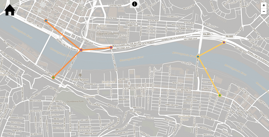
These clusters span multiple intervening roads and the Monongahela River. They’re an extreme example, created by a fairly large ε. But seeing clusters like this made us realize that for Accident Explorer to be as meaningful as we wanted it to be, we needed to modify DBSCAN even more.
Creating the cluster algorithm, take two
So we introduced two new factors to our algorithm: street name recognition and a two-part ε. Now instead of a single ε, we have a big ε and a small ε, and we define neighbors like this:
After a number of trials, we concluded that big ε=0.25mi and small ε=0.125mi were the best values to deal with urban vs rural accident density.
Big ε detects significant rural clusters, while street name recognition limits its effects in urban areas. Small ε detects significant urban clusters, and its lack of street name recognition allows accidents on frontage roads, on/off ramps, and just past intersections to be clustered with accidents on the main road.
Our modified algorithm also applies a form of the minimum neighbor count (K in DBSCAN) by only allowing clusters of more than three accidents to be displayed on the map.
We’re pleased by the effectiveness of our new algorithm, but its usefulness is still limited by a problem fundamental to big data projects: the integrity of the data.
Dirty data
The most significant issue is the street names.
The NHTSA tried to head off these problems using an extensive specification. For the street names, there are a lot of rules: don’t use street numbers; spell out the street type; prefix state highways with SR-…
But as we know, the specification doesn’t control what the data looks like: for example, there are street type abbreviations all over the FARS data. We had to process the data so that our algorithm’s street name matching wouldn’t be thrown off by non-meaningful differences like Av vs Ave vs Avenue.
And an incomplete specification turned out to be the least of our street name problems.
Missing clusters
Many, many streets in the United States are known by multiple names and/or numbers. Madison is full of examples: McKee Road is County PD, University Avenue is County MS, and the Beltline changes from US 12/14 to US 12/14/18/151 to US 12/18 in the space of about three miles.
Accidents in the FARS data come with latitude and longitude, so we’re able to place them along a road fairly precisely. But to fully account for multiple street names and numbers, we’d have to be able to identify which of a street’s possible names and numbers are appropriate at the accident’s location.
We don’t have this data, and putting it together would need much more time and labor than we’re able to give a demo like Accident Explorer.
Since we’re not able to account for this street naming problem, accidents which are too far apart for small-ε clustering but close enough for big-ε clustering aren’t clustered if they are reported with different street names.
Here’s one example from an earlier version: if you remove the street name recognition requirement from Accident Explorer, clusters end up controlled primarily by big ε. Using this version of the algorithm and the 2010-2012 data, there’s a four-accident cluster in Elizabeth, New Jersey:
This is a legitimate cluster by our complete algorithm’s standards: the accidents are all on the same street, and all can be transitively matched using ε=0.25mi.
But in the 2010-2012 production version of Accident Explorer, with street name matching added, this cluster was gone. Why?
Take a look at the data when street matching isn’t applied:
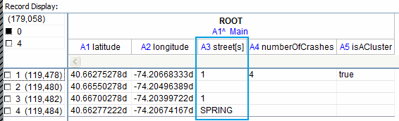
The street in question is Spring Street, a.k.a. US 1/9. Two of the accidents reported the street name as 1, one accident reported the street name as Spring, and one didn’t report a street name at all.
So when street name matching was implemented, the four-accident cluster became one two-accident cluster and two one-accident clusters. Accident Explorer only shows clusters with three or more accidents.
And that’s how the Elizabeth cluster disappeared.
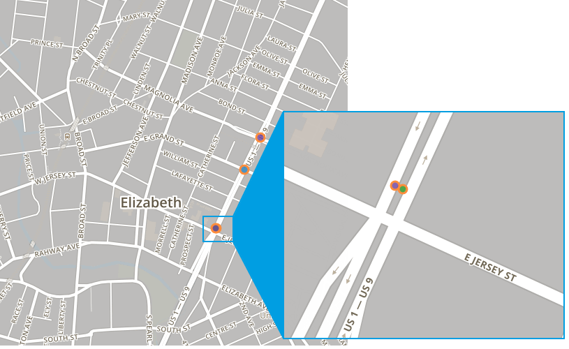
Adding the 2013 data contributed a new accident, partially restoring the cluster based on small-ε clustering:
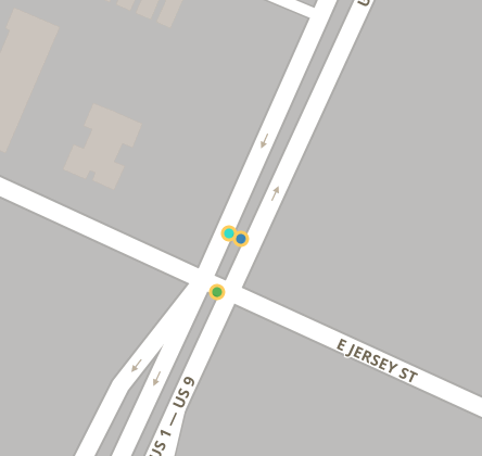
But this cluster is still incomplete, because the other two accidents are still missing. They’re too far away for small-ε clustering, but they aren’t clustered using big ε either.
The accident at Spring and E Grand is within 0.25mi of the visible cluster but it doesn’t have a street name match, and the accident at Spring and Magnolia is more than 0.25mi from the other US-1 accident.
Conclusion
Accident Explorer is a demo of MIOedge’s unsupervised machine learning. But it’s also an object lesson in how your results are only as good as the data you use to get them.
A significant contributor to the missing cluster problem is that we only have the FARS data, and the FARS data lists each street under just one name. If we had other data sources that covered the same accidents as FARS, but used different street names, we could make a more sophisticated algorithm for the clustering process.
This more advanced algorithm could identify when multiple sources are describing the same accident, even if the street names are different. Then, crucially, the algorithm could use all of the street names assigned to the accident for big-ε-based clustering. By synthesizing information, we could rediscover some missing clusters even without a comprehensive street-names-and-numbers database.
This is a major benefit of a context database: the more data you have, the more complete your picture can get. Adding data to Accident Explorer—whether it’s more sources for traffic accidents, or population and traffic density estimates—would only create a more accurate picture of fatal vehicle accident clusters in the US.
So always think about the completeness of the data that you’re basing your decisions on. And drive safely.

 For Data Migration